ICME 2017 HW1
Contents
|
Overview
In this homework, we will bridge information from the electronic scale to the nanoscale by calibrating a MEAM potential to specific DFT data. MEAM potentials can be calibrated with a number of physical quantities, however by downscaling our end goal of modeling the plastic behavior of our material, we can narrow it down to two very important quantities, the energy-volume (EV) curves and the generalized stacking fault energy (GSFE) curve. We can use other quantities to validate our potential.
There are two parts to this homework,
- Density Functional Theory (DFT) calculations
- Interatomic Modified Embedded Atom Method (MEAM) potential development
All necessary input files and scripts are provided here or in /scratch/ICME_2017/Homework1/ . Move any of these files to your own directory (and make a backup copy) before trying to perform any simulations.
Use /scratch/"Your Directory" for best results, especially if your job reads/writes much data.
Write a full report that follows a journal article manuscript format (include figures and tables in the text).
Upon completion, submit a .pdf and .doc(x) file of your report. Be sure to also include the requested files and plots from each section of the homework.
Part 1 - DFT Calculations
Objective
In Part 1, we will calculate the energy-volume (EV) and generalized stacking fault energy (GSFE) curves for our target material. For this course, we will use Vienna Ab initio Software Package (VASP) or Quantum Espresso to run the DFT calculations.
Environment Setup
VASP Setup
A video tutorial on getting started with VASP is available here. To run a VASP simulation, five files are needed. The names of the files (except the executable) are fixed for VASP as it simply looks for files with these names.
- vasp_5212_talon The vasp executable
- INCAR Controls the kind of solution performed
- KPOINTS Defines the frequency-space grid used to solve the equations - similar to a mesh
- POSCAR Positions of the atoms in the system
- POTCAR Defines the atomic potential used for your material
You can will find the executable, the various INCAR files, the KPOINTS file, and the appropriate POTCAR in /scratch/ICME_2017/Homework1/ . You will need to modify the INCAR and KPOINTS through each of the sections. The POSCAR will also vary for each assignment - in most cases it is created by the run scripts.
Quantum Espresso Setup
To run a Quantum Espresso simulation, three files are needed. The names of the files are not fixed for Quantum Espresso, as you will specify the input file and pseudopotential file directly. You can obtain Quantum Espresso by following the download link on the code page. A video tutorial on how to get started with Quantum Espresso is available here.
- pw.x or pw.exe The plane wave module executable from Quantum Espresso
- *.in The input script defining the type of calculation, the atomic positions and potential, and the K-points
- *.UDF The pseudopotential file - defines the electronic potential used for your material
Run Scripts
You will need the run scripts for creating the EV curves and the GSFE curves. Make sure to get the correct version for either VASP or Quantum Espresso.
You will also need the helper program evfit. As long as you run it on a Mississippi State cluster or shared memory system, the compiled program in /scratch/ICME_2017/Homework1/ will work. If you run it elsewhere, you may need to compile it from the source.
Batch Scripts
The version of VASP available at Mississippi State will only run on the HPC cluster machines. To submit jobs on these systems, you will need a PBS script. Make sure you have the two pbs scripts ev.pbs, gsfe.pbs from /scratch/ICME_2017/Homework1/ .
You can also modify these PBS scripts for Quantum Espresso, but Quantum Espresso can also be run locally or on your personal computer.
Energy-Volume (EV) curves (upscaling for MEAM calibration)
Walk-through
A video tutorial for this section can be found here.
Step 1
If using VASP, modify the batch script ev.pbs to reflect your material. Change the line beginning #PBS -Nto name your simulation. Change the final line,
./ev_curve fcc 4.08to reflect your structure and initial guess for the lattice parameter.
If you are using Quantum Espresso, you will need to create three input files named *.ev.in where * is the name of each structure in all lowercase (fcc, bcc, hcp). For an example input script, see the code page. You can set each of these up for each lattice structure by looking at the Quantum Espresso documentation for the plane wave input file.
Step 2
Modify the run script, ev_curve , to control the range and number of points generated, as well as the type of equation of state used to generate the results.
The lattice spacings are controlled by the section of code
 # Set the range and number of points generated
low=`echo 0.8\*$3 | bc` 		# Sets the lower bound to 80% of guess
high=`echo 1.2\*$3 | bc`		# Sets the upper bound to 120% of guess
step=`echo "($high-$low)/20" | bc -l`	# Sets stepsize such that 20 points are created
The equation of state is specified where the evfit routine is called. The "4" corresponds to the fourth equation of state, see the documentation for more information on your options.
# Once VASP has been run for each lattice parameter in the range
# Run evfit routine with equation of state 4
cat <<! | ./evfit
$1
4
EvsA
evfit.4
!
Step 3
Run the simulations!
If you are at Mississippi State using VASP, first you will need to make sure the correct software is setup when you log on to the cluster. To do this, make sure the following lines are added to /home/YOUR_USERNAME/.bashrc above the line stating " # All non-interactive shells will exit on the next line. "
swsetup pbs:intel:openmpiThen, logon to one of the the HPC clusters (eg. Raptor) and type:
qsub ev.pbsYour job will be added to the queue. You can check the status with
qstat -u YOUR_USERNAMEIf you are using Quantum Espresso, simply execute the command below, replacing the names with your material and lattice parameter guess, as in Step 1.
./ev_curve fcc 3.61
Step 4
The script will create several output files.
SUMMARY will give an overview of the values obtained using the specified equation of state.
The raw data obtained can be found in EvsA (energy vs. lattice parameter) and EvsV (energy vs. volume).
Step 5 (optional): Python Post-processing
Multiple python scripts have been created to assist in post-processing the data generated by the (Code: Quantum Espresso)simulations and SUMMARY / evfit / EvsV/ EvsV files generated through the process of completing the homework. The codes will parse the necessary files and generate plots and use the matplotlib python library to generate figures. There are currently 5 different files that can be used depending on what information is required. It is not necessary to use these codes to to the post-processing, but they are a useful tool.
- The EvA EvV plot.py code generates plots for the energy vs volume and energy vs lattice parameter curves for any set of EvsA an EvsV files generated by the ev_curve.bash script.
- The Convergence plots.py code generates plots for the convergency study from the
SUMMARYfiles. - The EOS plot.py code plots the difference in the energy values found from DFT and from the chosen EOS.
- The EOS comp plot.py code plots the energy vs lattice parameter curve from DFT and EOS fitting for multiple equations of state and compares the difference between each equation of state to values found directly from DFT.
- The Ecut conv.py code plots the values found from the ecut convergence studies.
All of the codes require some user modification (some more than others), but overall they greatly simplify processing all of the data generated from the simulations.
Homework Assignment
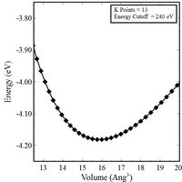
1. Plot energy (E) vs. volume (V) and energy (E) vs. atomic separation (A) curves for your material in its reference crystal structure (set PREC = Normal, in VASP).
2. For your material's reference crystal structure, perform a KPOINT convergence study (set PREC = Normal, in VASP). Choose the KPOINT grid that reaches a converged solution (think of this as a mesh refinement).
- a. Plot lattice parameter vs. KPOINT grid
- b. Plot bulk modulus vs. KPOINT grid
- c. Plot cpu time vs. KPOINT grid
- d. (Optional) If you are using Quantum Espresso, you should also insure that your results are converged with respect to the energy cutoff (ecutwfc). Note that the energy cutoff value is in Rydberg, rather than eV as in VASP.
3. Provide a thorough analysis of the four (4) equations of state (EOS) used for deriving the equilibrium lattice constant, bulk modulus, and cohesive energy e.g. How does changing the range of the simulation change the derived parameters?
4. Come up with final converged KPOINT grid and plot final E-V and E-A curves (set PREC = High, in VASP).
5. Provide a final set of values using the converged KPOINT and EOS of your choice. This data will be use for calibrating the MEAM potential.
6. Report on your results
- a. Copy all summary files to your ICME group folder
- b. Copy final E-A curves (EvsA) for each of the main structures (fcc, bcc, hcp) to your ICME group folder
Generalized Stacking Fault Energy (GSFE) curves (upscaling for MEAM calibration)
Walk-through
Step 1
Edit the script, gsfe_curve.py , to reflect the DFT code you will be using.
#
### EDIT THIS PARAMETER FOR CODE IN USE
# 'qe' - Quantum Espresso
# 'vasp' - VASP
dft = 'qe'
If using VASP, modify the batch script
gsfe.pbs to reflect your system. Change the line beginning #PBS -Nto name your simulation. Change the final line,
./gsfe_curve.py fcc 3.63 partialto reflect your structure and the ground state lattice parameter.
If you are using Quantum Espresso, edit the script, gsfe_curve.py , with your material and pseudopotential.
Step 2
If using VASP, modify the pbs script, gsfe.pbs to choose the stacking fault to use.
./gsfe_curve.py fcc 3.63 partialchange the last term to set the type of stacking fault to use. To see what each of the stacking faults are available for your material, simply run the GSFE script from the command line with
./gsfe_curve.pyThe code will prompt you for the required inputs, and describe the stacking fault types using a face and direction in Miller indices. The name in parentheses will tell you the name to use in your PBS script or command.
Step 3
Modify the python script, gsfe_curve.py , to control how many points are generated.
##### STACKING FAULT PARAMETERS - USER EDIT IF NEEDED #####
# Number or location of simulated points. It MUST start with 0.
#fault_points = [0.0, 1./6., 1./3.]
fault_points = np.linspace(0,1,19)
You can use the commented line ( #fault_points = np.linspace(0,1,19) ) to create evenly spaced points, or the line above it to specify specific points.
The displacement is normalized here - points should range from 0 to 1, and start with 0.
Step 4
Run the simulations!
If you are at Mississippi State, logon to one of the the HPC clusters (eg. Raptor) and typeqsub gsfe.pbsYour job will be added to the queue. You can check the status with
qstat -u YOUR_USERNAMEGSFE jobs can often take a few to several hours, depending on the number of points, and k-point density. Plan accordingly!
If you are using Quantum Espresso, simply run the command below, replacing the material, structure, lattice parameter, and dislocation type with the ones for your system, as in Steps 1 and 2.
./gsfe_curve fcc 3.61 partial
Step 5
Gather the results.
GSFE_SUMMARY contains the displacement (in units of the lattice parameter) vs. GSFE values in mJ/m^2.
Homework Assignment
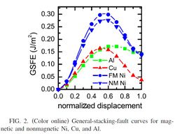
1. Produce a GSFE curve for your material.
- a. Take care with the slip system and direction you use! You will need to know this when fitting your MEAM potential. For FCC, we typically look at the Shockley partial curve, {111}<112>.
- b. Use the converged KPOINT and energy cutoff values obtained from the previous section.
2. Report your results.
- a. Plot the change in energy vs. upper atom displacement.
- b. Copy final GSFE curve(s) to your group folder.
Additional examples for performing the necessary simulations are found by clicking the on the respective image below:
 |
 |
|---|
Part 2 - MEAM Potential Development
Objective
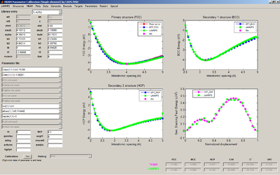
For this portion of the assignment, you will use the MEAM Parameter Calibration (MPC) tool to fit a MEAM potential.
MEAM Potential Calibration/Validation
Fit the modified embedded atom method (MEAM) model and generate a new MEAM potential for your material by using the property values calculated above from the DFT results. Tutorial videos for using the MPC tool can be found here and here.
The calibration will include values calculated by DFT: Equilibrium nearest neighbor distance/lattice parameter, cohesive energy, GSFE curve, and the elastic moduli (sometimes the surface formation energy for (111) surface is used but not in this homework). Elastic constants can be checked with literature results (experimental values in Table III page 15 of Mehl et al.).
1. Using the MEAM Potential Calibration (MPC) routine determine the MEAM constants by comparing the energy versus atomic separation (E-A) plots from DFT and LAMMPS:
- a. Using DFT results set alat, esub, and bulk
- b. Calibrate the MEAM constants to single crystal elastic moduli found in the literature
- c. Calibrate the MEAM parameters to the GSFE curve obtained from DFT using Cmin, asub, b1, and b3
- d. Plot a comparison of the E-A for the different cases on one plot
- e. Plot a comparison of the GSFE from DFT and GSFE from MPC
2. Conduct a validation check by comparing one of the MEAM calculations available in MPC to a literature value.
3. Sensitivity analysis
- a. Vary several of the parameters (one at a time) up to 50% to show the sensitivity of the parameters on the E-A curve and GSFE curve
- b. Plot the comparisons for E-A and GSFE curves for the different cases on one plot each (one containing the E-A sensitivities and one containing the GSFE sensitivities)
4. Report your results
- a. Place a screenshot of the final fitting routine and parameters in your group folder
5. Add a section or sections on improving the tutorial by adding/modifying the ICME webpage used for:
- a. VASP
- b. LAMMPS
 |
|---|
License
By using the codes provided here you accept the the Mississippi State University's license agreement. Please read the agreement carefully before usage.
Additional Guides
References
- ↑ C. Brandl, P. M. Derlet, and H. Van Swygenhoven, General-stacking-fault energies in highly strained metallic environments: Ab initio calculations, PHYSICAL REVIEW B 76, 054124 (2007)